Available materializations
Views and tables and incremental models, oh my! In this section we’ll start getting our hands dirty digging into the three basic materializations that ship with dbt. They are considerably less scary and more helpful than lions, tigers, or bears — although perhaps not as cute (can data be cute? We at dbt Labs think so). We’re going to define, implement, and explore:
- 🔍 views
- ⚒️ tables
- 📚 incremental model
👻 There is a fourth default materialization available in dbt called ephemeral materialization. It is less broadly applicable than the other three, and better deployed for specific use cases that require weighing some tradeoffs. We chose to leave it out of this guide and focus on the three materializations that will power 99% of your modeling needs.
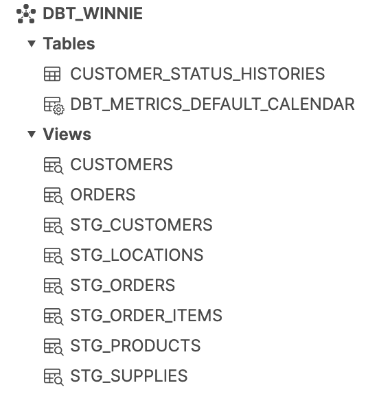
Views and Tables are the two basic categories of object that we can create across warehouses. They exist natively as types of objects in the warehouse, as you can see from this screenshot of Snowflake (depending on your warehouse the interface will look a little different). Incremental models and other materializations types are a little bit different. They tell dbt to construct tables in a special way.
Views
- ✅ The default materialization in dbt. A starting project has no configurations defined for materializations, which means everything is by default built as a view.
- 👩💻 Store only the SQL logic of the transformation in the warehouse, not the data. As such, they make a great default. They build almost instantly and cost almost nothing to build.
- ⏱️ Always reflect the most up-to-date version of the input data, as they’re run freshly every time they’re queried.
- 👎 Have to be processed every time they’re queried, so slower to return results than a table of the same data. That also means they can cost more over time, especially if they contain intensive transformations and are queried often.
Tables
- 🏗️ Tables store the data itself as opposed to views which store the query logic. This means we can pack all of the transformation compute into a single run. A view is storing a query in the warehouse. Even to preview that data we have to query it. A table is storing the literal rows and columns on disk.
- 🏎️ Querying lets us access that transformed data directly, so we get better performance. Tables feel faster and more responsive compared to views of the same logic.
- 💸 Improves compute costs. Compute is significantly more expensive than storage. So while tables use much more storage, it’s generally an economical tradeoff, as you only pay for the transformation compute when you build a table during a job, rather than every time you query it.
- 🔍 Ideal for models that get queried regularly, due to the combination of these qualities.
- 👎 Limited to the source data that was available when we did our most recent run. We’re ‘freezing’ the transformation logic into a table. So if we run a model as a table every hour, at 10:59a we still only have data up to 10a, because that was what was available in our source data when we ran the table last at 10a. Only at the next run will the newer data be included in our rebuild.
Incremental models
- 🧱 Incremental models build a table in pieces over time, only adding and updating new or changed records.
- 🏎️ Builds more quickly than a regular table of the same logic.
- 🐢 Initial runs are slow. Typically we use incremental models on very large datasets, so building the initial table on the full dataset is time consuming and equivalent to the table materialization.
- 👎 Add complexity. Incremental models require deeper consideration of layering and timing.
- 👎 Can drift from source data over time. As we’re not processing all of the source data when we run an incremental model, extra effort is required to capture changes to historical data.
Comparing the materialization types
| view | table | incremental | |
|---|---|---|---|
| 🛠️⌛ build time | 💚 fastest — only stores logic | ❤️ slowest — linear to size of data | 💛 medium — builds flexible portion |
| 🛠️💸 build costs | 💚 lowest — no data processed | ❤️ highest — all data processed | 💛 medium — some data processed |
| 📊💸 query costs | ❤️ higher — reprocess every query | 💚 lower — data in warehouse | 💚 lower — data in warehouse |
| 🍅🌱 freshness | 💚 best — up-to-the-minute of query | 💛 moderate — up to most recent build | 💛 moderate — up to most recent build |
| 🧠🤔 complexity | 💚 simple - maps to warehouse object | 💚 simple - map to warehouse concept | 💛 moderate - adds logical complexity |
🔑 Time is money. Notice in the above chart that the time and costs rows contain the same results. This is to highlight that when we’re talking about time in warehouses, we’re talking about compute time, which is the primary driver of costs.